Plan Equivalence
Two inference plans are equivalent if they produce identical token sequences under identical model and constraint semantics.
Definition (-Equivalence)
Two plans are -equivalent if logits differ by at most over the valid candidate set and produce identical decoded outputs.
Lemma: Dense and Sparse Equivalence
Let denote the valid token set. Dense masked scoring:
Sparse scoring:
Then:
Roofline Regime Analysis
Dense head compute:
Sparse head compute:
Sparse dominates when:
Amortized Query Hypothesis
We model decoder state as:
Full transformer recomputation may provide limited incremental information when margins are large. Define margin:
Routing decision — refine if:
Otherwise use amortized scoring.
Planner Routing as a Contextual Bandit
At decoding step , the planner observes a context vector and selects an execution plan . We define a scalar loss:
and seek to minimize .
Oracle and Regret
Define the per-step oracle action:
and dynamic regret:
For stationary regimes, define the best fixed plan:
with static regret:
Linear Contextual Bandit
Assume realizability: , with . LinUCB/linear Thompson sampling achieves sublinear regret of the form:
where and hides logarithmic factors.
Nonstationarity and Variation Budget
To capture policy churn, define a variation budget:
Sliding-window or restart-based bandits can achieve dynamic regret bounds of the form:
under standard boundedness assumptions.
Connection to Margin-Based Routing
The threshold router from the amortization section is a finite policy class when is discretized. This enables expert-style learning over with regret for candidate thresholds.
Compiler Integration: Plan Selection in MLIR / StableHLO
Modern inference stacks already compile model graphs through MLIR and StableHLO. LLM-QP can therefore be implemented as a compiler pass that introduces multiple equivalent execution plans and selects among them using a cost model.
Logical vs Physical Plans
We define a logical operator: DecodeStep(query, constraint_state) which expresses the semantics of a single constrained decoding step. Physical implementations include:
- Dense projection head
- Sparse adjacency scoring
- Amortized query update
- Amortized update with rerank
- Full recomputation (refinement)
Plan Expansion Pass
During compilation the planner expands the logical node into candidate physical plans:
DecodeStep
  -> DenseHead
  -> SparseHead
  -> AmortizedHead
  -> AmortizedHead + Rerank
Cost Model
Each plan is annotated with an estimated cost covering kernel latency estimates, memory bandwidth usage, refinement probability, and device utilization. The cost function follows:
Rewrite Rule
if cost(SparseHead) < cost(DenseHead):
    use SparseHead
else:
    use DenseHead
In practice this is implemented using MLIR pattern rewrites or XLA custom calls.
Runtime Adaptation
Runtime telemetry (margins, branching factor, cache state) feeds back into the cost model. The compiler therefore emits a small routing kernel that chooses the implementation at runtime. This hybrid compile-time / runtime planning architecture allows LLM-QP to reuse existing compiler infrastructure while enabling adaptive execution.
Visualizations
Planner Pseudocode
LinUCB for Plan Selection
Let and feature dimension . Maintain per-action matrices and vectors initialized as , . At each step :
- Observe context .
- For each action , estimate and compute:
- Choose (loss-minimization).
- Execute plan , observe loss .
- Update and .
Expert-Over-Thresholds Routing
Discretize thresholds and define policies . Maintain weights initialized uniformly. At each step :
- Observe context and compute each expert’s suggested action .
- Sample an expert index proportional to weights (or pick for greedy).
- Execute , observe loss .
- Update weights using exponential weighting:where is an unbiased loss estimate.
This realizes regret against the best threshold policy in hindsight under standard assumptions.
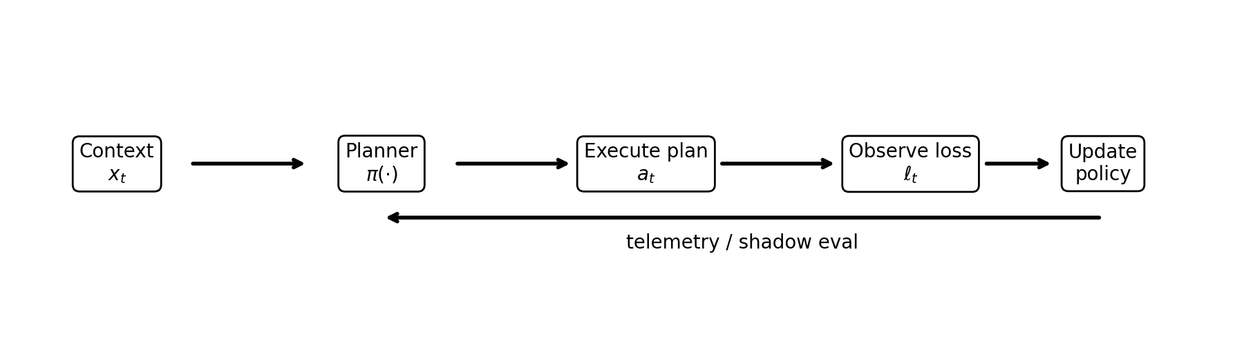
End-to-End System Architecture
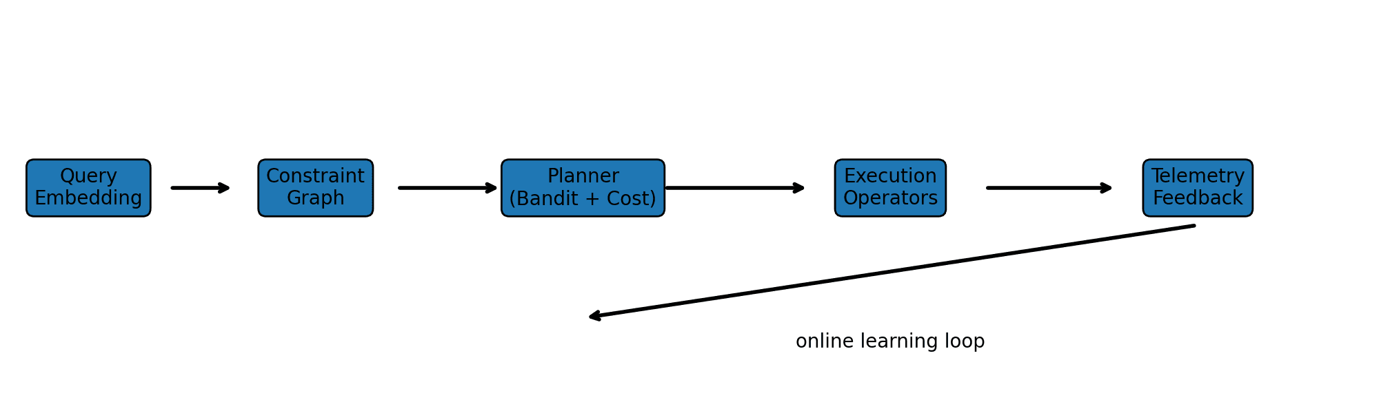
The pipeline operates as follows:
- Query embedding produces a representation of the decoding state.
- The constraint graph defines valid token transitions.
- The planner selects an execution plan using contextual signals.
- The chosen operator executes the step.
- Telemetry feeds back to update routing decisions.
Minimal Reproducible Benchmarks
We provide a portable benchmark harness (synthetic, deterministic) that instantiates the cost models and routing policies used throughout the paper. The suite outputs: (i) dense vs sparse crossover vs , (ii) amortized vs full recomputation crossover vs decode length, and (iii) router regret relative to an oracle policy (threshold router).
The harness now runs here, in the browser. Drag the parameters; the three figures below are recomputed live from the model’s own equations, and the router is a real LinUCB instance learning against the oracle.
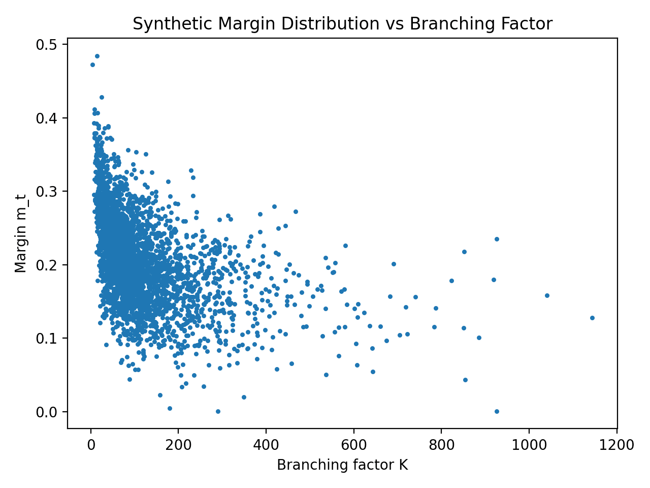
Sparse scoring wins while K < |V|
Constrained decoding scores only the valid tokens. The dense head costs 2d|V| no matter what; the sparse head costs 2dK, where K is the number of legal tokens right now. Move the model dimension and vocabulary and watch the crossover sit exactly at K = |V|.
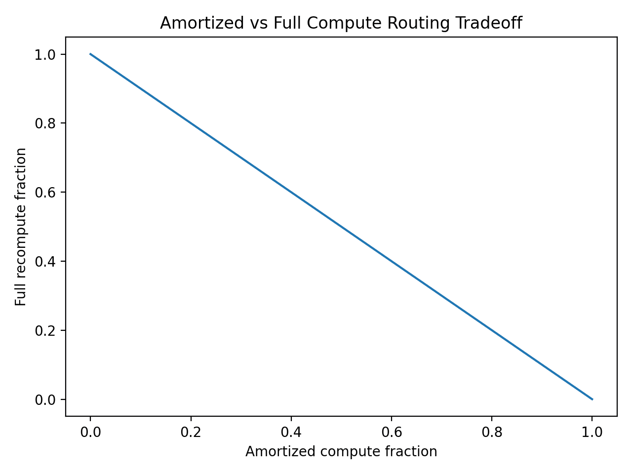
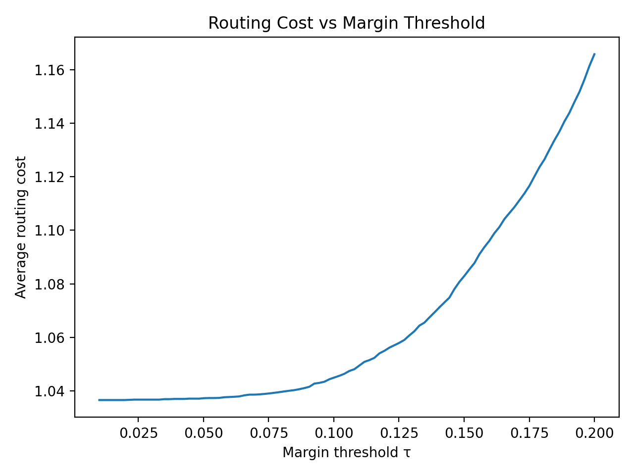
Amortize when the model is confident
If the top token is far ahead of the runner-up (a large margin), the next step probably has the same answer, so skip the full recompute. Refine only when the margin falls below the threshold τ. Drag τ: at τ = 0 the model trusts every step (cheapest, riskiest); at τ = 1 it refines always and collapses onto full recompute.
The router learns to route
A real LinUCB contextual bandit (Appendix A, running in your browser) sees each step’s context — how many tokens are valid, how confident the model is — and picks a plan. It is paid the true cost and updates. Watch cumulative regret against the hindsight oracle bend over and flatten: that bend is the convergence the paper claims, and nobody told the router the answer.
Deterministic given the seed. The router converges to within a few percent of the unbeatable oracle and leaves both fixed policies behind — and it learns that the conservative dense head is dominated, so it almost never picks it.